Understanding dc motor curves and temperature: Part 2

by Dan Montone, PITTMAN Motors/AMETEK Precision Motion Control, Harleysville, PA

Motor performance changes with temperature. Understanding the effects of heat and temperature changes will help in selecting the right motor for an application.

How much can motor performance change under a given set of conditions?

Here we look at a specific example of changes in motor performance using a specific set of conditions. The initial data are:

• Terminal Voltage, (V_T) 24 V
• No Load Speed, (n₀) 3160 RPM
• No Load Current, (I₀) 0.30 A
• Locked Rotor Torque, (T_LR) 2.88 Nm
• Locked Rotor Current, (I_LR) 40.7 A
• Terminal Resistance, (R_mt) 0.59 Ω
• Voltage Constant, (K_E) 0.071 V/(rad/s)
• Torque Constant, (K_T) 0.071 Nm/A
• Motor Regulation, (R_m) 1111 RPM/Nm
• Initial Motor Temperature, (Ѳ_i) 25°C
• Stabilized Armature Temperature, (Ѳ_f) 125°C
• Armature Temperature Rise, (Ѳ_r) 100°C

Conditions:

• Initial motor data was created using a rapid dynamometer test at a room temperature of 25°C
• With a consistent load on the motor, the armature temperature stabilized to 125°C
• No heat sink or forced airflow was used
• The motor was operated open loop (no feedback to regulate shaft output power)
• Power supply used – regulated, 50A max output with low output impedance
• Copper motor windings
• Strontium ferrite (ceramic) permanent magnets

With a stabilized armature temperature rise of 100°C, terminal resistance will be higher and magnetic flux density will be lower compared with the initial motor temperature of 25°C.  This will result in a change in R_mt, K_T and K_E.

The calculations that follow assume that the permanent magnet and wound armature temperatures are identical.  The motor armature, which is the part of the machine carrying electric current, will always be at a higher temperature than the permanent magnets.  In practice, the actual change in K_T, K_E, and motor regulation will be less pronounced than what’s demonstrated in the following example.

Estimated Motor Characteristics at an Elevated Temperature of 125°C

Increased Terminal Resistance
R_mt(f)  = R_mt(i) x [1 + α_conductor (Ѳ_f – Ѳ_i)]
R_mt(f)  =  0.59Ω x [1 + 0.0040 (125°C – 25°C)]
R_mt(f)  =  0.83Ω

Decreased Torque and Voltage Constant (K used for both K_E and K_T assuming SI units)
K_(f)  =  K_(i) x [1 + α_magnet (Ѳ_f – Ѳ_i)]
K_(f)  =  0.071 V/rad/s x [1 + (-0.0020)(125°C – 25°C)]
K_(f)  =  0.057 V/rad/s or Nm/A

Decreased Locked Rotor (Stall) Current
I_LR = V_T / R_mt(f)
I_LR = 24V / 0.83Ω
I_LR = 28.92A

Decreased Locked Rotor (Stall) Torque
T_LR = I_LR x K_T(f)
T_LR = 28.92A x 0.057Nm/A
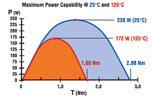
T_LR = 1.65Nm

Increased No Load Speed
n₀ = 9.5493 x [(V_T – I₀ x R_mt(f)) / K_E(f)]
n₀ = 9.5493 x [(24V – 0.30A x 0.83 Ω) / 0.057V/rad/s]
n₀ = 3979 RPM

Increased Motor Regulation
R_m = n₀ / T_LR
R_m = 3979 RPM / 1.65 Nm
R_m = 2412 RPM / Nm

It’s interesting to note how much the performance changes with a given increase in motor temperature.  Although the analysis is helpful in understanding the phenomenon, it’s by no means perfect.  There are a few things to keep in mind. For example:

1) We assumed a stabilized 100°C rise on all components of the motor.  In practice, the various motor components will stabilize at different temperatures, with the wound motor armature being the highest.

2) The temperature coefficient for the magnetic material was an average used for that material.  In reality, different grades of a particular material class will have values that deviate slightly from the average.

3) The true thermal model of a DC motor is extremely complex.  It’s very difficult to obtain exact values theoretically, as there are just too many variables to consider.

The first approximation analysis, however, is very helpful in applying the motor and understanding its limitations in a particular application.

Motor Constants and Maximum Output Power
Rarely, if ever, is a motor operated at the maximum power point for long.  With the exception of small, low-power motors, most cannot be operated continuously at the maximum power point without exceeding the temperature rating.  The equations below can be used to determine the power at any point on the motor curve and maximum output power.

Equation 6a – Motor Output Power (at any point)
P_out = ω x T

Equation 6b – Maximum Output Power
P_max = 0.25 x ω₀ x T_LR

Equation 6c – Maximum Output Power (Theoretical)
P_max = 0.25 x (V_T² / R_mt)

Equations 6b and 6c illustrate the effect of motor resistance on the output power capability of the machine.  Although not intuitive by looking at equation 6b, a higher winding resistance at an elevated temperature is the main culprit in reducing the maximum output power capability of the motor.  Even though magnetic flux is reduced, this is equally compensated by an increase in motor speed (due to reduced K_E).  If the resistance stayed the same, even a decrease in magnetic flux density will not significantly change the maximum output power of the machine.  In reality, the higher resistance (R_mt) combined with the reduced magnetic flux density (lower K_T) reduces the locked rotor torque much more than just a reduction in magnetic flux density alone, which accounts for the reduction in maximum output power.

Maximum output power @ 25°C
P_max(i) = 0.25 x ω₀ x T_LR
P_max(i)  = 0.25 x 331 rad/s x 2.88 Nm
P_max(i)  = 238 W

Maximum output power @ 125°C
P_max(f) = 0.25 x ω₀ x T_LR
P_max(f)  = 0.25 x 417 rad/s x 1.65 Nm
P_max(f)  = 172 W

The maximum power at the elevated temperature is approximately 70% of the maximum power at room temperature.  This is a significant change, and it’s a direct consequence of the increased motor resistance.  Equation 6c will give results that are within 1 or 2% of the numbers above.  This equation is helpful in rapidly estimating the maximum power capability of any DC motor.

Published Data – Motor curves come in many varieties
Most DC motor performance charts will show at least two curves; speed versus torque and current versus torque.  Manufacturers may decide to display the information in slightly different ways and also supply other information such as output power and efficiency curves.

An example motor curve removes all other variables and assumes the motor is tested with a fixed terminal voltage using a low impedance power supply and progressively loaded with a dynamometer. The test is performed as quickly as possible to minimize motor temperature rise.  If the motor being tested is a small sub-fractional horsepower motor, the dynamometer may load the motor until shaft speed hits zero or close to zero RPM.  In the case of larger motors, the dynamometer may be set to progressively load the motor to approximately the maximum power point.  The remainder of the curve may then be extrapolated.   The resulting data in either case are (theoretically) straight-line speed versus torque and current versus torque curves.

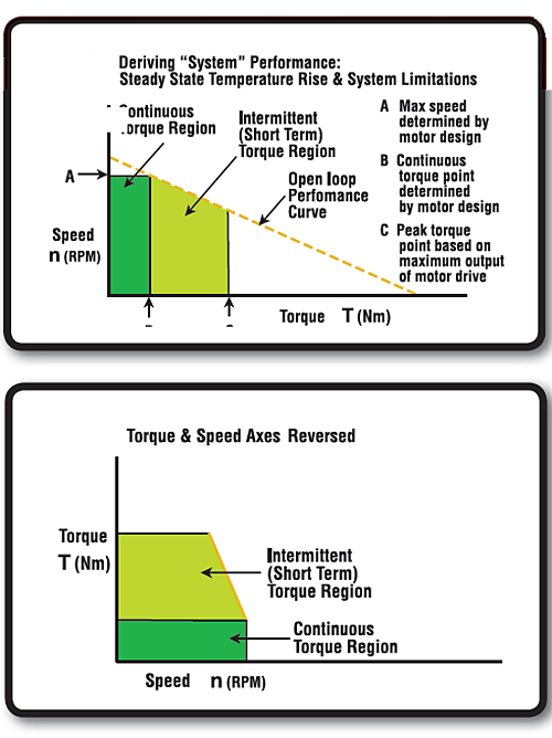
Some manufacturers, in particular those that supply complete servo systems, may present performance curves as a “blend” of information that includes system-level limitations. The limitations considered can include many things such as continuous current capability, peak current capability, drive/amplifier power limitations, maximum DC bus voltage, maximum motor temperature ratings, motor saturation, and mechanical speed limitations.  Many manufacturers may illustrate motor torque on the “Y” axis and speed on the “X” axis.  The example curves in Figure 4 illustrate how data might look if factors such as maximum rotational speed, maximum temperature rise, and peak drive current are considered.  No matter how the data is published or what other system factors are considered, the motor parameters R_mt, K_T, and K_E are critical for understanding the true capabilities of the motor.

Another factor to keep in mind when evaluating various performance curves is that actual test conditions may not always be obvious.  Different suppliers will publish different information.  In the case where the motors are tested rapidly on a dynamometer (to minimize temperature rise), this method tends to be very consistent and provides a good baseline.  The disadvantage is that the results don’t represent worst case conditions.

If the motors are tested at the maximum rated temperature, the user will better understand the motor capability when used in applications where motor temperature will stabilize at a value significantly higher than room temperature.  The disadvantage is that there are many other variables that can skew the test results such as method of temperature measurement, motor mounting (causing a heat sinking effect), air flow around the motor, etc.  Some motor manufacturers will test their motors under the worst case condition; a motor stabilized to full rated temperature with no heat sinking or forced air flow.  There are no strict guidelines dictating how a manufacturer should present the performance data. The important thing to remember when evaluating the information is to ask the right questions.

Overall Motor Construction and Heat Transfer
Mechanical structure affects the heat transfer characteristics in the motor.  In a DC motor with a mechanical commutator and brushes, the copper windings are wound in slots around the armature.  The heat generated by the copper windings on the armature will conduct through the armature laminations and to the motor shaft and bearing system.  Through convection, the heat will also migrate across the air gap to the permanent magnets and housing where it will ultimately be dissipated into the surrounding environment.  Although some of the heat transfer takes place using direct conduction through the lamination stack to the bearing system and housing, much of the heat generated will flow via the air gap and through the magnets.

In the case of a brushless DC motor, the copper windings are wound in slots (in a slotted brushless motor) or formed against magnetic back iron (in a slotless brushless motor) and constructed as part of the inside surface of the motor housing.  This construction allows a direct thermally conductive path from the heat generating copper to the motor housing where it will be dissipated into the environment. The permanent magnets in a brushless motor are on the rotating part of the machine.

In either case, it will be difficult if not impossible to predict the temperature rise of individual components without empirical testing, but one thing is certain; the thermal rise of individual components (hot spots within the motor) will be different between a brush and brushless motor, all other factors remaining equal.

There’s No Substitute for Application Testing
The purpose of the preceding discussion and the calculation examples is to gain a better understanding of how motor performance changes with temperature. There is no substitute for testing and validating the motor under application conditions.  A proper theoretical treatment would not be feasible due to the number of variables and assumptions involved. However, the example calculations can serve as a first approximation to get an idea of the magnitude of possible change.

The best way to understand motor performance under actual operating conditions is to simulate the application as closely as possible while collecting temperature data over time with a data acquisition system.  Various parts of the motor should be monitored using thermocouples attached to bearings, end bells, windings (in the case of a brushless motor), magnets (in the case of a brush motor) and the motor housing. And remember to always discuss design criteria with an applications engineer.

Reprint info >>

AMETEK Precision Motion Control
www.ametek.com